7. Quantization and optimization
In deploying neuron network, the accuracy and throughput (inference speed) are critical targets. To achieve high accuracy and high speed, for some networks, mix precision inference is essential.
The mixed-precision method of TPU-MLIR is searching layers in neural network that are not suitable for low-bit quantization to generate a quantize table, which is used to specify these layers to use higher-bit quantization in the model_deploy stage. This chapter will first introduce the current full int8 symmetric quantization of TPU-MLIR, and then explain how to use the existing quantize table automatic generation tools in TPU-MLIR.
7.1. TPU-MLIR Full Int8 Symmetric Quantization
TPU-MLIR adopts full int8 symmetric quantization by default, where full int8 means that all operators, except for those that the compiler defaults to floating-point operations (such as layernorm), are quantized to int8. This section introduces how to use the TPU-MLIR full int8 symmetric quantization tool.
After generating the corresponding MLIR file for the model using the model_transform command as instructed in the previous tutorial, if you want to perform int8 symmetric quantization on the model,
you also need to generate a calibration table cali_table using the run_calibration command. How to use the parameters of the run_calibration command for different types of models to ensure
the generated quantized model has good accuracy will be provided in detailed guidance below.
7.1.1. run_calibration Process Introduction
The quantization part of the following figure (:ref:calibration) shows the overall process of the current run_calibration , which includes the automatic mixed-precision module search_qtable , the automatic calibration method selection module search_threshold , cross-layer weight equalization module weight_equalization,
and bias correction module bias_correction, etc. In the following sections, we will provide the usage details of the above methods based on actual situations.
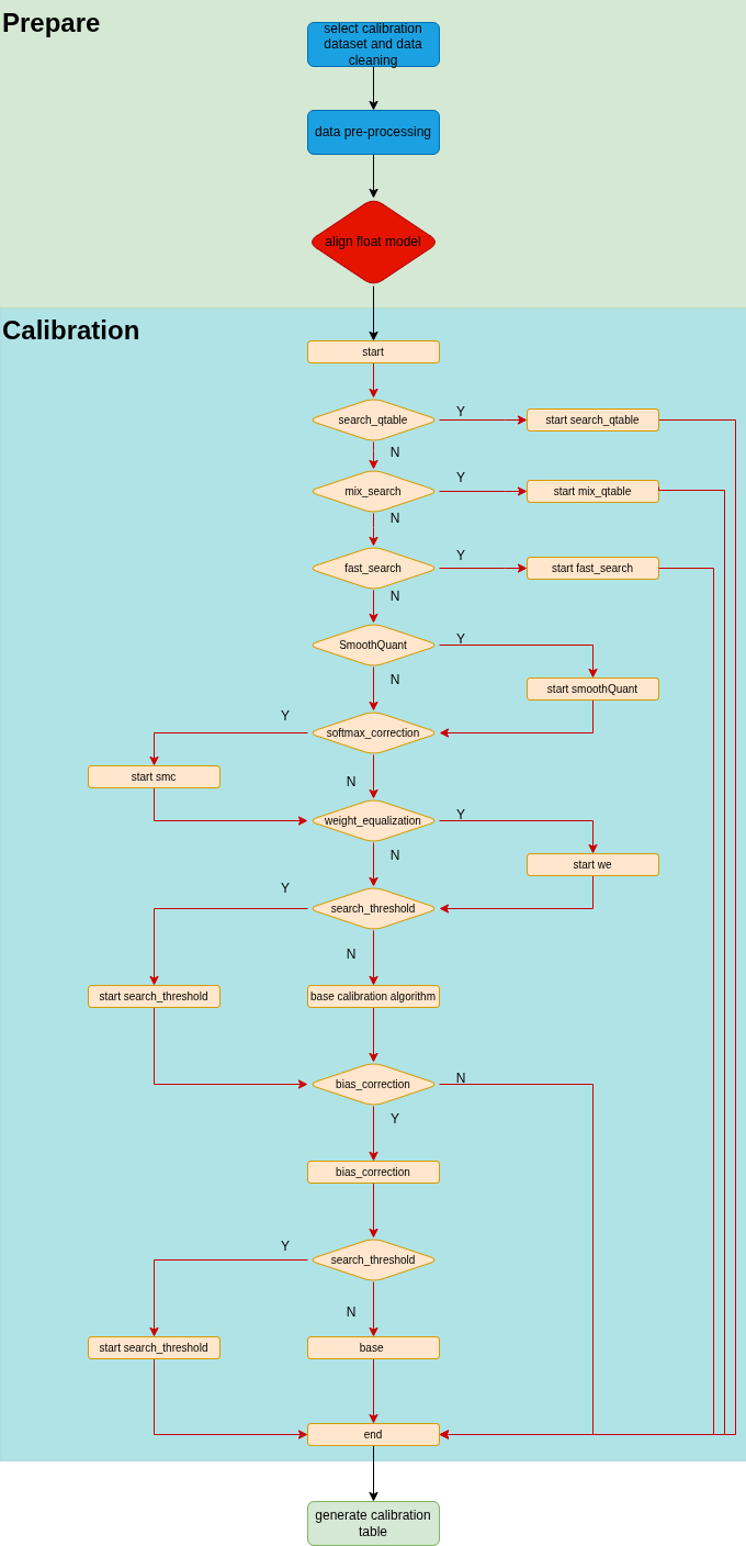
Fig. 7.1 run_calibration process
7.1.2. run_calibration Parameter Introduction
The table below provides an introduction to the parameters of the run_calibration command.
parameter |
description |
|---|---|
mlir_file |
mlir file |
sq |
open SmoothQuant |
smc |
open softmax_correction |
we |
open weight_equalization |
bc |
open bias_correction |
dataset |
calibration dataset |
data_list |
sample list |
input_num |
number of calibration sample |
inference_num |
the number of images required for the inference process with search_qtable and search_threshold is set to 30 by default |
bc_inference_num |
the number of images required for the inference process with bias correction is set to 30 by default |
tune_list |
the list of sample used for tuning |
tune_num |
the number of images for tuning |
histogram_bin_num |
specify the number of histogram bins for KLD calculation, default is 2048 |
expected_cos |
expect the similarity between the mixed-precision model output of search_qtable and the floating-point model output, with a value range of [0,1], default is 0.99 |
min_layer_cos |
the lower bound of similarity between the quantized output and the floating-point output of the layer in bias_correction; compensation is required for the layer when it falls below this threshold, with a value range of [0,1], default is 0.99 |
max_float_layers |
set the number of floating-point layers for search_qtable, default is 5 |
processor |
processor type, default is bm1684x |
cali_method |
select the calibration mode; if this parameter is not added, the default is KLD calibration. “percentile9999” uses the 99.99 percentile as the threshold. “max” uses the absolute maximum value as the threshold. “use_torch_observer_for_cali” uses torch’s observer for calibration. “mse” uses octav for calibration. |
fp_type |
search_qtable floating-point layer data type |
post_process |
post-processing path |
global_compare_layers |
specify the global contrastive layers, for example, layer1,layer2 or layer1:0.3,layer2:0.7. |
search |
specify the search type, which includes search_qtable, search_threshold, and false. The default is false, which means search is not enabled |
transformer |
whether it is a transformer model, in search_qtable, if it is a transformer model, a specific acceleration strategy can be assigned, default is False |
quantize_method_list |
the calibration method used for searching in search_qtable, default is MSE, with selectable range being MSE, KL, MAX, Percentile9999 |
benchmark_method |
specify the similarity calculation method of search_threshold, with the default being cosine similarity (cos) |
kurtosis_analysis |
Specify the generation of the kurtosis of the activation values for each layer |
part_quantize |
Specify partial quantization of the model. The calibration table (cali_table) will be automatically generated alongside the quantization table (qtable). Available modes include N_mode, H_mode, or custom_mode, with H_mode generally delivering higher accuracy |
custom_operator |
Specify the operators to be quantized, which should be used in conjunction with the aforementioned custom_mode |
part_asymmetric |
When symmetric quantization is enabled, if specific subnets in the model match a defined pattern, the corresponding operators will automatically switch to asymmetric quantization |
mix_mode |
Specify the mixed-precision types for the search_qtable. Currently supported options are 8_16 and 4_8 |
cluster |
Specify that a clustering algorithm is used to detect sensitive layers during the search_qtable process |
quantize_table |
the mixed-precision quantization table from search_qtable |
o |
cali_table output path |
debug_cmd |
debug command |
debug_log |
log output level |
7.1.3. The Use of run_calibration Parameters Introduction
Based on the user’s needs and their understanding of the model itself and quantization, we have provided targeted ways to use the run_calibration parameters in different situations.
scenario |
description |
quantization speed |
calibration method |
recommended method |
|---|---|---|---|---|
case1 |
initial model quantization |
insensitive |
unclear |
search_threshold |
case2 |
initial model quantization |
/ |
clear |
cali_method directly selects the corresponding calibration method |
case3 |
initial model quantization |
sensitive |
unclear |
the cali_method selects a fixed calibration method; for details on choosing a specific calibration method, refer to the subsequent sections |
case4 |
after model quantization, the accuracy on the bm1684 processor does not meet the requirements |
/ |
/ |
open sq, smc, we and bc methods |
case 1: When you perform the initial quantization on your model, which is the first time you use the run_calibration command, you may not be clear
about the calibration method that is best suited for your current model and you may not be sensitive to the quantization speed.
In this case, it is recommended to use the search_threshold method. This method can automatically select the calibration method that is most suitable
for your current model and output the calibration table cali_table generated by this method to the output path you specify. It will also generate a log file Search_Threshold,
which records the quantization information for different calibration methods. The specific operation is as follows:
$ run_calibration mlir.file \
    --dataset data_path \
    --input_num 100 \
    --processor bm1684x \
    --search search_threshold \
    --inference_num 30 \
    -o cali_table
Notes:1.At this point, it is necessary to select the processor parameter, which corresponds to the processor platform on which the model is intended to be deployed. The current default is bm1684x.
2. inference_num corresponds to the number of inference data required for the search_threshold process (this data will be extracted from the dataset you provide).
The larger the inference_num, the more accurate the search_threshold result, but the longer the quantization time required. Here, the default for inference_num is set to 30, which can be customized according to the actual situation.
case2: When quantizing your model for the first time, you already know which calibration method is suitable for the model or you want to try specific method/methods. At this point, you can directly choose a fixed calibration method based on the cali_method parameter. The specific operation is as follows:
$ run_calibration mlir.file \
    --dataset data_path \
    --input_num 100 \
    --cali_method mse \
    -o cali_table
Notes:1.when the cali_method parameter is not specified, the default KLD calibration method will be used. 2.currently, the cali_method supports other five options: mse, max, percentile9999, aciq_gauss and aciq_laplace.
case3: When you are sensitive to quantization time and wish to generate the calibration table cali_table as quickly as possible, but you are unsure how to choose a calibration method, it is recommended to select a fixed calibration method based on the cali_method parameter.
In comparison to the quantization speed of TPU-MLIR V1.8, the V1.9 version shows a 100% speed improvement for individual calibration methods, resulting in an average time reduction of around 50%. The acceleration effect is significant.
In the V1.9 version, mse is the fastest calibration method on average. When selecting a calibration method, you can consider the following empirical conclusions:
1.For non-transformer models without attention structure, mse is a suitable calibration method. Here is a specific operation guide:
$ run_calibration mlir.file \
    --dataset data_path \
    --input_num 100 \
    --cali_method mse \
    -o cali_table
You can also choose the default KLD calibration method. Here is a specific operation guide:
$ run_calibration mlir.file \
    --dataset data_path \
    --input_num 100 \
    -o cali_table
If neither of the above two methods meets the accuracy requirements, you may need to consider adopting a mixed precision strategy or a hybrid threshold method. More detailed information on these approaches can be found in the subsequent section.
2.When your model is a transformer model that includes an attention structure, you can choose the mse calibration method. If the mse calibration method does not produce satisfactory results, you can then consider trying the max calibration method. Here is a specific operation guide:
$ run_calibration mlir.file \
    --dataset data_path \
    --input_num 100 \
    --cali_method max \
    -o cali_table
If the max method also fails to meet the requirements, at this point, you may need to adopt a mixed precision strategy. You can then try the mixed precision methods that will be introduced later.
Apart from the overall selection rules mentioned above, here are some specific details for choosing calibration methods:1.If your model is a YOLO series object detection model, it is recommended to use the default KLD calibration method, for yolo26 series models, it is recommended to use mse or percentile9999 calibration method.2.If your model is a multi-output classification model,
it is also recommended to use the default KLD calibration method.
case4: When your model is deployed on the bm1684 processor and the full int8 quantized model obtained through the methods mentioned above has poor accuracy,
you can try enabling SmoothQuant (sq), softmax correction (smc), cross-layer weight equalization (we) and bias correction (bc). To do this, simply add the sq, smc, we and bc parameters to the original command.
If you have used search_threshold for searching, the operations for adding sq, smc, we and bc are as follows:
$ run_calibration mlir.file \
    --sq \
    --smc \
    --we \
    --bc \
    --dataset data_path \
    --input_num 100 \
    --processor bm1684 \
    --search search_threshold \
    --inference_num 30 \
    --bc_inference_num 100 \
    -o cali_table
If you choose a fixed calibration method using cali_method , for example, using mse , to add the sq, smc, we and bc methods, the specific operation is as follows:
$ run_calibration mlir.file \
    --sq \
    --smc \
    --we \
    --bc \
    --dataset data_path \
    --input_num 100 \
    --processor bm1684 \
    --cali_method mse \
    --bc_inference_num 100 \
    -o cali_table
If you are using the default KLD calibration method, simply remove the cali_method parameter.
Notes:1.Make sure to specify the processor parameter as bm1684. 2.The bc_inference_num parameter is the number of data samples required when using the bc quantization method (these samples will be extracted from the dataset you provide), so the number of images should not be too few.
3.The sq, smc, we and bc methods can be used independently. If you choose only the we method, simply omit the sq, smc and bc parameters in the operation. 4. Shape calculation ops will be found and set as float in model_name_shape_ops qtable saved in the current directory, the content of this file can be merged by hand with following mix-precision setting files.
7.2. Overview of TPU-MLIR Mixed Precision Quantization
TPU-MLIR provides model mixed precision quantization methods, with its core step being the acquisition of a quantize_table ,hereafter referred to as qtable that records operator names and their quantization types.
TPU-MLIR provides two paths for obtaining the qtable:
For typical models, TPU-MLIR provides an experience-based pattern-match method.
For special or atypical models, PU-MLIR provides mixed precision quantization methods search_qtable and fp_forward tools to generate the qtable.
The following four section will provide detailed introductions to these four mixed precision methods.
7.3. pattern-match
The pattern-match method is integrated into run_calibration and does not require explicit parameter specification.
Currently, there are two type of models for which experience qtable is provided: one is the YOLO series, and the other is the Transformer series (e.g., BERT).
After obtaining the cali_table , if the model matches an existing pattern, a qtable will be generated in the path/to/cali_table/ folder.
Before calibration, purpose of every op is judged, if it is calculating shape or position, it is treated as special pattern, and will be set float and included in qtable.
7.3.1. YOLO Series Automatic Mixed Precision Method
Currently pattern-match method supported YOLO models include YOLOV5, V6, V7, V8, V9, V10, V11, V12 and yolo26.
YOLO series models are classic and widely used. When exporting models through official support,
post-processing branches with significantly different numerical values are often merged for output, leading to large accuracy loss when quantizing the model to full INT8.
Due to the similar structural features of YOLO series models (i.e., a three-level maxpool structure),
pattern-match automatically identifies whether the model belongs to the YOLO series. If so, operators in the post-processing part will further be recognized and set as float in qtable.
This qtable can be manually merged with the following hybrid precision configurations for use in model_deploy.
Example of YOLOv8 model output:
1['top.MaxPool', 'top.MaxPool', 'top.MaxPool', 'top.Concat'] (Name: yolo_block) is a subset of the main list. Count: 1
2The [yolov6_8_9_11_12] post-processing pattern matches this model. Block count: 1
3The [yolov6_8_9_11_12] post-processing pattern is: ['top.Sub', 'top.Add', 'top.Add', 'top.Sub', 'top.MulConst', 'top.Concat', 'top.Mul', 'top.Concat']
4The qtable has been generated in: path/to/cali_table/qtable !!!
7.3.2. Transformer Series Automatic Mixed Precision Method
Currently pattern-match method supported Transformer series models include BERT, EVA, DeIT, Swin, CSWin, ViT, and DETR.
If the above modules are identified, SiLU, GELU and LayerNorm after Add operators will be set as non-quantized. For ViT, MatMul after Softmax/GELU operators will be identified. For EVA, MatMul after SiLU→Mul and Add operators will be identified. For Swin, Permute before Reshape→LayerNorm, Add and Depth2Space operators will be identified. For DETR, all operators except Conv, Scale, Reshape, and MatMul after LayerNorm/Reshape will be set as non-quantized. These operators are set as non-quantized to generate the qtable.
7.4. 1. search_qtable
search_qtable is a mixed precision feature integrated into run_calibration. When full int8 quantization precision does not meet the requirements, mixed precision method are needed, meaning that some operators are set to perform floating-point operations.
This section takes mobilenet-v2 as example to introduce how to use search_qtable.
This section requires the tpu_mlir python package.
7.4.1. Install tpu_mlir
$ pip install tpu_mlir[all]
# or
$ pip install tpu_mlir-*-py3-none-any.whl[all]
7.4.2. Prepare working directory
Please obtain tpu-mlir-resource.tar from SDK package and unzip it, and rename the folder to tpu_mlir_resource :
$ tar -xvf tpu-mlir-resource.tar
$ mv regression/ tpu-mlir-resource/
Preparation and Usage Instructions for Single-Input Model Calibration Dataset (Taking mobilenet-v2 as an Example) :
Establish a directory structure
Create a
mobilenet-v2directory, and put both model files and image files into themobilenet-v2directory. You can get mobilenet_v2.pt from tpu-mlir-resource.tar (provided in SDK package).Prepare the calibration dataset
–dataset uses the ILSVRC2012 dataset, which contains 1000 types of images, with 1000 images in each type. Here, only 100 images from these are used for calibration
Dataset format
Users can create a dataset directory by themselves and directly place image files (such as JPEG, PNG, etc.) into this directory. run_calibration.py will automatically read the image and, based on the model input parameters such as shape, mean, and scale, automatically complete the preprocessing and format conversion into a numpy array as the model input. However, multi-input models must use structured data (such as npz), because only these formats can clearly distinguish the name, shape, and dtype of each input.
The operation is as follows:
Single-Input Model:
1 $ mkdir mobilenet-v2 && cd mobilenet-v2
2 $ mv path/to/mobilenet_v2.pt .
3 $ cp -rf tpu_mlir_resource/dataset/ILSVRC2012 .
4 $ mkdir workspace && cd workspace
Preparation and Usage Instructions for multi-input Model Calibration Dataset (taking bert_base_squad_uncased-2.11.0 as an example) :
Establish a directory structure
Create the directory ‘bert_base_squad_uncased-2.11.0’ and put both the model file and the image file into the directory ‘bert_base_squad_uncased-2.11.0’.
Prepare the calibration dataset
The –dataset uses the SQuAD dataset, which contains multiple samples, and each sample contains multiple input data.
Dataset format
Users can create a dataset directory by themselves. Under the directory, npz files must be placed. Each npz file represents a sample and contains all the input keys (the name, shape, and dtype must be consistent with the model input). Pictures cannot be placed directly.
multi-input Model:
1 $ mkdir bert_base_squad_uncased-2.11.0 && cd bert_base_squad_uncased-2.11.0
2 download bert_base_squad_uncased-2.11.0.onnx
3 download SQuAD/mlir
4 download squad_uncased_data.npz
5 $ mkdir workspace && cd workspace
7.4.3. Accuracy test of float anf int8 models
7.4.3.1. Step 1: To F32 mlir
$ model_transform \
    --model_name mobilenet_v2 \
    --model_def ../mobilenet_v2.pt \
    --input_shapes [[1,3,224,224]] \
    --resize_dims 256,256 \
    --mean 123.675,116.28,103.53 \
    --scale 0.0171,0.0175,0.0174 \
    --pixel_format rgb \
    --mlir mobilenet_v2.mlir
multi-input Model:
$ model_transform.py \
    --model_name bert_base_squad_uncased-2.11.0 \
    --model_def ../bert_base_squad_uncased-2.11.0.onnx \
    --test_input ../squad_uncased_data.npz \
    --input_shapes '[[1, 384], [1, 384], [1, 384]]' \
    --test_result bert_base_squad_uncased-2.11.0_top_outputs.npz \
    --mlir bert_base_squad_uncased-2.11.0.mlir
7.4.3.2. Step 2: Gen calibartion table
Here, we use the mse method for calibration.
$ run_calibration.py mobilenet_v2.mlir \
    --dataset ../ILSVRC2012 \
    --input_num 100 \
    --cali_method mse \
    -o mobilenet_v2_cali_table
multi-input Model:
$ run_calibration.py bert_base_squad_uncased-2.11.0.mlir \
     --dataset ../SQuAD/mlir \
     --input_num 10 \
     --tune_num 0 \
     --debug_cmd mse \
     -o bert_base_squad_uncased-2.11.0.calitable
7.4.3.3. Step 3: To F32 bmodel
$ model_deploy \
    --mlir mobilenet_v2.mlir \
    --quantize F32 \
    --processor bm1684 \
    --model mobilenet_v2_1684_f32.bmodel
7.4.3.4. Step 4: To INT8 model
$ model_deploy \
    --mlir mobilenet_v2.mlir \
    --quantize INT8 \
    --processor bm1684 \
    --calibration_table mobilenet_v2_cali_table \
    --model mobilenet_v2_bm1684_int8_sym.bmodel
7.4.3.5. Step 5: Accuracy test
classify_mobilenet_v2 is a python program, to run mobilenet-v2 model.
Test the fp32 model:
$ classify_mobilenet_v2.py \
    --model_def mobilenet_v2_bm1684_f32.bmodel \
    --input ../ILSVRC2012/n02090379_7346.JPEG \
    --output mobilenet_v2_fp32_bmodel.JPEG \
    --category_file ../ILSVRC2012/synset_words.txt
The classification information is displayed on the output image. The right label sleeping bag ranks first.
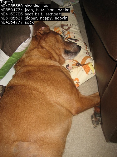
Fig. 7.2 Execution Performance of classify_mobilenet_v2 in FP32
Test the INT8 model:
$ classify_mobilenet_v2.py \
    --model_def mobilenet_v2_bm1684_int8_sym.bmodel \
    --input ../ILSVRC2012/n02090379_7346.JPEG \
    --output mobilenet_v2_INT8_sym_bmodel.JPEG \
    --category_file ../ILSVRC2012/synset_words.txt
The classification information is displayed on the output image. The right label sleeping bag ranks second.

Fig. 7.3 Execution Performance of classify_mobilenet_v2 in INT8
7.4.4. To Mix Precision Model
After int8 conversion, do these commands as beflow.
7.4.4.1. Step 1: Execute the search_qtable command
The search_qtable feature is currently integrated into the run_calibration process. Therefore, to use it, you only need to add the relevant parameters to the run_calibration command.
The parameters related to search_qtable in run_calibration are explained as follows:
Name |
Required? |
Explanation |
|---|---|---|
(None) |
Y |
mlir file |
dataset |
N |
Directory of input samples. Images, npz or npy files are placed in this directory |
data_list |
N |
The sample list (cannot be used together with “dataset”) |
processor |
Y |
The platform that the model will use. Support bm1688, bm1684x, bm1684, cv186x, cv183x, cv182x, cv181x, cv180x |
fp_type |
N |
Specifies the type of float used for mixing precision. Support auto,F16,F32,BF16. Default is auto, indicating that it is automatically selected by program |
input_num |
N |
The number of samples used for calibration |
inference_num |
N |
The number of samples used for inference, default 30 |
max_float_layers |
N |
The number of layers set to float, default 5 |
tune_list |
N |
The sample list for tune threshold |
tune_num |
N |
The number of samples for tune threshold, default 5 |
post_process |
N |
The user defined prost process program path, default None |
expected_cos |
N |
Specify the minimum cos value for the expected final output layer of the network. The default is 0.99 |
debug_cmd |
N |
Specifies a debug command string for development. It is empty by default |
global_compare_layers |
N |
global compare layers, for example: |
search |
Yes |
Specify the search type, which includes |
transformer |
N |
Is it a transformer model? In |
quantize_method_list |
N |
the calibration method used for searching in |
quantize_table |
Yes |
qtable output path |
pre_qtable |
n |
qtable as the base to search from, replace the default pattern match and shape ops as qtable |
calibration_table |
Yes |
cali_table output path |
search_qtable supports user defined post process programs post_process_func.py. It can be placed in the current project directory or in another location, if it is placed in another location, you need to specify the full path of the file in the post_process . The post process function must be named PostProcess , the input data is the output of the network and the output data is the post-processing result. Create the post_process_func.py file with the following sample contents:
def PostProcess(data):
    print("in post process")
    return data
search_qtable can customize the calibration method with mixed thresholds, controlled by the parameter quantize_method_list. By default, only the MSE calibration method is used for the search. If you want to use a mixed search with KLD and MSE, set the parameter quantize_method_list to KL,MSE.
search_qtable has an acceleration strategy for transformer models. If the model is a transformer model with an attention structure, you can set the parameter transformer to True.
Use search_qtable to search for layers with significant loss. Note that it is recommended to use bad cases for the search.
In this example, 100 images are used for quantization, 30 images are used for inference, and a mixed search using KLD and MSE calibration methods is performed. Execute the command as follows:
$ run_calibration.py mobilenet_v2.mlir \
    --dataset ../ILSVRC2012 \
    --input_num 100 \
    --inference_num 30 \
    --expected_cos 0.99 \
    --quantize_method_list KL,MSE \
    --search search_qtable \
    --transformer False \
    --processor bm1684 \
    --post_process post_process_func.py \
    --quantize_table mobilenet_v2_qtable \
    --calibration_table mobilenet_v2_cali_table \
The final output after execution is printed as follows:
the layer input3.1 is 0 sensitive layer, loss is 0.004858517758037473, type is top.Conv
the layer input5.1 is 1 sensitive layer, loss is 0.002798812150635266, type is top.Scale
the layer input11.1 is 2 sensitive layer, loss is 0.0015642610676610547, type is top.Conv
the layer input13.1 is 3 sensitive layer, loss is 0.0009357141882855302, type is top.Scale
the layer input6.1 is 4 sensitive layer, loss is 0.0009211346574943269, type is top.Conv
the layer input2.1 is 5 sensitive layer, loss is 0.0007767164275293004, type is top.Scale
the layer input0.1 is 6 sensitive layer, loss is 0.0006842551513905892, type is top.Conv
the layer input128.1 is 7 sensitive layer, loss is 0.0003780628201499603, type is top.Conv
......
run result:
int8 outputs_cos:0.986809 old
mix model outputs_cos:0.993372
Output mix quantization table to mobilenet_v2_qtable
total time:667.644282579422
success search qtable
Above, int8 outputs_cos represents the cosine similarity between network outputs of int8 model and float model; mix model outputs_cos represents the cosine similarity between network outputs of mix model and float model; total time represents the search time is 667 seconds.
In addition,this program generates a quantization table mobilenet_v2_qtable, the context is as below:
# op_name   quantize_mode
input3.1 F32
input5.1 F32
input11.1 F32
input13.1 F32
input6.1 F32
In the table, the first column represents the corresponding layer, and the second column represents the type. Supported types are F32/F16/BF16/INT8. search_qtable will determine
the number of mixed precision layers in the qtable based on the user-defined expected_cos parameter value. For example, if the expected_cos parameter value is equal to 0.99,
the number of mixed precision layers in the qtable corresponds to the minimum number of mixed precision layers required to achieve that level of model output comparison.
Of course, the number of mixed precision layers in the table will be limitted based on the number of model operators. If the minimum number of mixed precision layers exceeds the limitation,
only the limited quantity of mixed precision layers will be taken. Additionally, a log file Search_Qtable will be generated with the following content:
 1INFO:root:quantize_method_list =['KL', 'MSE']
 2INFO:root:run float mode: mobilenet_v2.mlir
 3INFO:root:run int8 mode: mobilenet_v2.mlir
 4INFO:root:all_int8_cos=0.9868090914371674
 5INFO:root:run int8 mode: mobilenet_v2.mlir
 6INFO:root:layer name check pass !
 7INFO:root:all layer number: 117
 8INFO:root:all layer number no float: 116
 9INFO:root:transformer model: False, all search layer number: 116
10INFO:root:Global metrics layer is : None
11INFO:root:start to handle layer: input0.1, type: top.Conv
12INFO:root:adjust layer input0.1 th, with method KL, and threshlod 9.442267236793155
13INFO:root:run int8 mode: mobilenet_v2.mlir
14INFO:root:outputs_cos_los = 0.0006842551513905892
15INFO:root:adjust layer input0.1 th, with method MSE, and threshlod 9.7417731
16INFO:root:run int8 mode: mobilenet_v2.mlir
17INFO:root:outputs_cos_los = 0.0007242344141149548
18INFO:root:layer input0.1, layer type is top.Conv, best_th = 9.442267236793155, best_method = KL, best_cos_loss = 0.0006842551513905892
19.....
The log file first provides the custom parameters, including the calibration method
used for the mixed threshold quantize_method_list, the number of ops to be searched
all search layer number and whether it is a transformer model or not.
Then, it records the threshold obtained for each op under the given calibration methods
(in this case, MSE and KL) and provides the loss of similarity
(1 - cosine similarity) between the mixed-precision model using only the
corresponding threshold for that operation in int8 computation and the original
float model. It also includes the loss information of each operation output on
the screen side and the cosine similarity between the final mixed-precision
model and the original float model. Users can use the qtable output by the
program, or modify the qtable based on the loss information, and then generate
the mixed-precision model. After Search_Qtable is finished,
the optimal threshold will be updated to a new quantization table
new_cali_table.txt , stored in the current project directory, which needs to be
called when generating the mixed-precision model.
7.4.4.2. Step 2: Gen mix precision model
$ model_deploy \
    --mlir mobilenet_v2.mlir \
    --quantize INT8 \
    --processor bm1684 \
    --calibration_table new_cali_table.txt \
    --quantize_table mobilenet_v2_qtable \
    --model mobilenet_v2_bm1684_int8_mix.bmodel
7.4.4.3. Step 3: Test accuracy of mix model
$ classify_mobilenet_v2 \
    --model_def mobilenet_v2_bm1684_int8_mix.bmodel \
    --input ../ILSVRC2012/n02090379_7346.JPEG \
    --output mobilenet_v2_INT8_mix_bmodel_1.JPEG \
    --category_file ../ILSVRC2012/synset_words.txt
The classification information is displayed on the output image. The right label sleeping bag ranks first.

Fig. 7.4 Execution Performance of classify_mobilenet_v2 in the Mixed Precision Model
7.5. 2. fp_forward
For specific neural networks, some layers may not be suitable for quantization due to significant differences in data distribution. The “Local Non-Quantization” allows you to add certain layers before, after, or between other layers to a mixed-precision table. These layers will not be quantized when generating a mixed-precision model.
In this section, we will continue using the example of the YOLOv5s network mentioned in Chapter 3 and demonstrate how to use the Local Non-Quantization to quickly generate a mix-precision model.
The process of generating FP32 and INT8 models is the same as in Chapter 3. Here, we focus on generating mix-precision model and the accuracy testing.
For YOLO series models, the last three convolutional layers often have significantly different data distributions, and adding them manually to the mixed-precision table can improve accuracy. With the Local Non-Quantization feature, you can search for the corresponding layers from the Top MLIR file generated by model_transform and quickly add them to the mixed-precision table using the following command:
$ fp_forward \
    yolov5s.mlir \
    --quantize INT8 \
    --processor bm1684x \
    --fpfwd_outputs 474_Conv,326_Conv,622_Conv\
    -o yolov5s_qtable
Opening the file “yolov5s_qtable” will reveal that the relevant layers have been added to the qtable.
Generating the Mixed-Precision Model
$ model_deploy \
    --mlir yolov5s.mlir \
    --quantize INT8 \
    --calibration_table yolov5s_cali_table \
    --quantize_table yolov5s_qtable \
    --processor bm1684x \
    --test_input yolov5s_in_f32.npz \
    --test_reference yolov5s_top_outputs.npz \
    --tolerance 0.85,0.45 \
    --model yolov5s_1684x_mix.bmodel
Validating the Accuracy of FP32 and Mixed-Precision Models In the model-zoo, there is a program called “yolo” used for accuracy validation of object detection models. You can use the “harness” field in the mlir.config.yaml file to invoke “yolo” as follows:
Modify the relevant fields as follows:
$ dataset:
    imagedir: $(coco2017_val_set)
    anno: $(coco2017_anno)/instances_val2017.json

harness:
    type: yolo
    args:
        - name: FP32
        bmodel: $(workdir)/$(name)_bm1684_f32.bmodel
        - name: INT8
        bmodel: $(workdir)/$(name)_bm1684_int8_sym.bmodel
        - name: mix
        bmodel: $(workdir)/$(name)_bm1684_mix.bmodel
Switch to the top-level directory of model-zoo and use tpu_perf.precision_benchmark for accuracy testing, as shown in the following command:
$ python3 -m tpu_perf.precision_benchmark yolov5s_path --mlir --target BM1684X --devices 0
The accuracy test results will be stored in output/yolo.csv:
mAP for the FP32 model: mAP for the mixed-precision model using the default mixed-precision table:
Performance Testing
mAP for the mixed-precision model using the manually added mixed-precision table:
Parameter Description
Name |
Required? |
Explanation |
|---|---|---|
(None) |
Y |
mlir file |
processor |
Y |
The platform that the model will use. Support bm1688, bm1684x, bm1684, cv186x, cv183x, cv182x, cv181x, cv180x. |
fpfwd_inputs |
N |
Specify layers (including this layer) to skip quantization before them. Multiple inputs are separated by commas. |
fpfwd_outputs |
N |
Specify layers (including this layer) to skip quantization after them. Multiple inputs are separated by commas. |
fpfwd_blocks |
N |
Specify the start and end layers between which quantization will be skipped. Start and end layers are separated by colon, and multiple blocks are separated by space. |
fp_type |
N |
Specifies the type of float used for mixing precision. Support auto,F16,F32,BF16. Default is auto, indicating that it is automatically selected by program |
o |
Y |
output quantization table |
7.6. example of multi-input calibration dataset
For multi-input models, the calibration dataset can be saved in npz file, each npz contains one sample, and key of npz complies with model inputs, following is open_clip as example.
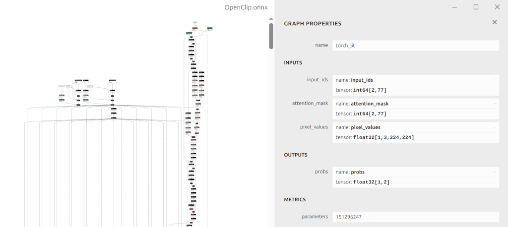
Fig. 7.5 OpenClip multi-input model
As there are three inputs in open_clip, one floating-point image and two integer idx and mask, you can create a calibration dataset following the function below:
def process_images(input_dir, output_file, image_size=(224, 224),
                  normalize=False, mean=None, std=None,samples=100,
                  channels_first=True, dtype='float32'):
    # Get all image files
    extensions = ['*.jpg', '*.jpeg', '*.JPG', '*.JPEG']
    image_files = []
    for ext in extensions:
        image_files.extend(Path(input_dir).glob(ext))

    image_files = list(set(image_files))  # Remove duplicates

    # Default normalization (ImageNet stats)
    if normalize:
        if mean is None:
            mean = [0.485, 0.456, 0.406]
        if std is None:
            std = [0.229, 0.224, 0.225]

    # Build transformation pipeline
    transform_list = [transforms.Resize(image_size)]

    if normalize:
        transform_list.extend([
            transforms.ToTensor(),
            transforms.Normalize(mean=mean, std=std)
        ])
    else:
        transform_list.append(transforms.ToTensor())

    transform = transforms.Compose(transform_list)

    # Process images
    filenames = []

    for i, img_path in enumerate(image_files):
        try:
            inputs={}
            img = Image.open(img_path).convert('RGB')
            tensor = transform(img)

            # Convert to numpy
            img_array = tensor.numpy()  # default float32
            img_array = np.expand_dims(img_array, axis=0)
            inputs['pixel_values'] = img_array
            inputs['input_ids'] = np.random.randint(0,100,size=(2,77))
            inputs['attention_mask'] = np.random.randint(0,1,size=(2,77))
            np.savez(f'{output_file}_{i}',**inputs)
            if i+1 >= samples:
                print(f"Processed {i + 1}/{len(image_files)} images")
                break
            filenames.append(str(img_path.name))

            if (i + 1) % 10 == 0:
                print(f"Processed {i + 1}/{len(image_files)} images")

        except Exception as e:
            print(f"Error processing {img_path}: {e}")


**NOTE: above code is for demo only, pre-processing must be aligned with training phase when creating npz files for calibration. Real calibration data can be captured during training.**