4. Compile the Torch Model

This chapter takes yolov5s.pt as an example to introduce how to compile and transfer an pytorch model to run on the BM1684X platform.

This chapter requires the tpu_mlir python package.

4.1. Install tpu_mlir

Go to the Docker container and execute the following command to install tpu_mlir:

$ pip install tpu_mlir[torch]
# or
$ pip install tpu_mlir-*-py3-none-any.whl[torch]

4.2. Prepare working directory

Please download tpu-mlir-resource.tar from Assets and unzip it, and rename the folder to tpu_mlir_resource :

$ tar -xvf tpu-mlir-resource.tar
$ mv regression/ tpu-mlir-resource/

Create a model_yolov5s_pt directory, and put both model files and image files into the model_yolov5s_pt directory.

The operation is as follows:

$ mkdir model_yolov5s_pt && cd model_yolov5s_pt
$ wget -O yolov5s.pt "https://github.com/sophgo/tpu-mlir/raw/master/regression/model/yolov5s.pt"
$ cp -rf tpu_mlir_resource/dataset/COCO2017 .
$ cp -rf tpu_mlir_resource/image .
$ mkdir workspace && cd workspace

4.3. TORCH to MLIR

The model in this example has a RGB input with mean and scale of 0.0,0.0,0.0 and 0.0039216,0.0039216,0.0039216 respectively.

The model conversion command:

$ model_transform \
    --model_name yolov5s_pt \
    --model_def ../yolov5s.pt \
    --input_shapes [[1,3,640,640]] \
    --mean 0.0,0.0,0.0 \
    --scale 0.0039216,0.0039216,0.0039216 \
    --keep_aspect_ratio \
    --pixel_format rgb \
    --test_input ../image/dog.jpg \
    --test_result yolov5s_pt_top_outputs.npz \
    --mlir yolov5s_pt.mlir

After converting to mlir file, a ${model_name}_in_f32.npz file will be generated, which is the input file of the model. It is worth noting that we only support static models, and the model needs to call torch.jit.trace() to generate a static model before compilation.

4.4. MLIR to F16 bmodel

Convert the mlir file to the bmodel of f16, the operation method is as follows:

$ model_deploy \
    --mlir yolov5s_pt.mlir \
    --quantize F16 \
    --processor bm1684x \
    --test_input yolov5s_pt_in_f32.npz \
    --test_reference yolov5s_pt_top_outputs.npz \
    --tolerance 0.99,0.99 \
    --model yolov5s_pt_1684x_f16.bmodel

After comiplation, a file named yolov5s_pt_1684x_f16.bmodel will be generated.

4.5. MLIR to INT8 bmodel

4.5.1. Calibration table generation

Before converting to the INT8 model, you need to run calibration to get the calibration table. Here is an example of the existing 100 images from COCO2017 to perform calibration:

$ run_calibration yolov5s_pt.mlir \
    --dataset ../COCO2017 \
    --input_num 100 \
    -o yolov5s_pt_cali_table

After running the command above, a file named yolov5s_pt_cali_table will be generated, which is used as the input file for subsequent compilation of the INT8 model.

4.5.2. Compile to INT8 symmetric quantized model

Execute the following command to convert to the INT8 symmetric quantized model:

$ model_deploy \
    --mlir yolov5s_pt.mlir \
    --quantize INT8 \
    --calibration_table yolov5s_pt_cali_table \
    --processor bm1684x \
    --test_input yolov5s_pt_in_f32.npz \
    --test_reference yolov5s_pt_top_outputs.npz \
    --tolerance 0.85,0.45 \
    --model yolov5s_pt_1684x_int8_sym.bmodel

After compilation, a file named yolov5s_pt_1684x_int8_sym.bmodel will be generated.

4.6. Effect comparison

Use the command detect_yolov5 path to perform object detection on the image.

Use the following codes to verify the execution results of pytorch/ f16/ int8 respectively.

The pytorch model is run as follows to get dog_torch.jpg:

$ detect_yolov5 \
    --input ../image/dog.jpg \
    --model ../yolov5s.pt \
    --output dog_torch.jpg

The f16 bmodel is run as follows to get dog_f16.jpg :

$ detect_yolov5 \
    --input ../image/dog.jpg \
    --model yolov5s_pt_1684x_f16.bmodel \
    --output dog_f16.jpg

The int8 asymmetric bmodel is run as follows to get dog_int8_sym.jpg :

$ detect_yolov5 \
    --input ../image/dog.jpg \
    --model yolov5s_pt_1684x_int8_sym.bmodel \
    --output dog_int8_sym.jpg

The result images are compared as shown in the figure (Comparison of TPU-MLIR for YOLOv5s compilation effect).

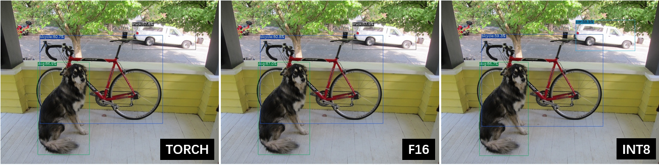
_images/yolov5s_pt.png — Fig. 4.1 Comparison of TPU-MLIR for YOLOv5s compilation effect

Due to different operating environments, the final performance will be somewhat different from Fig. 4.1.