1. Software and Hardware Framework of TPU#
As the following figure showd, a whole TPU application depends the cooperation of software and hardware:
For software, Host provides libsophon, driver software packs. Driver abstracts the mechanism of basic communication and resource management, defines function interfaces. Libsohpon implements varies of concrete functions for TPU inference, such as BMLib and TPU-RUNTIME. BMLib(libbmlib.so) wraps the driver interfaces for keeping compatiblity and portiblity of application, improving performance and simplicity of programming. TPU-RUNTIME(libbmrt.so) implements loading, management, execution, and so on.
For Hardware, TPU mainly consists of three engines: MCU, GDMA, TIU.
An A53 processor is used as MCU on BM1684X, which implements concrete operators by sending commands, communicating with driver, simple computation with firmware program. GDMA and TIU do the real computing related work. GDMA engine is used for transmitting data between Global Mem and Local Mem, moving data as 1D, Matrix, 4D formats, and TIU engine does the computing operations, including Convolution, Matrix Multiplication, Arithmetic Operations.

TPU Profile is a tool for visualizing the profile binary data in HTML formats which comes from the time information recording by the hardware modules called GDMA PMU and TPU PMU, the running time of key functions and the meta data in bmodel. The profile data generation is done during compiling bmodel, executing inference application which is disable by default, and can be enabled by setting environment variables.
This article mainly utilizes Profile data and TPU Profile tools to visualize the complete running process of the model, in order to provide readers with an intuitive understanding of the internal TPU.
2. Compile Bmodel#
(This operation and the following operations will use TPU MLIR)
Due to the fact that the profile data will save some layer information during compilation to the BModel, resulting in a larger volume of the BModel, it is disabled by default. The opening method is to call the model_deploy.py with the ‘– debug’ option. If this option is not used during compilation, some data obtained by enabling profile during visualization may be missing.
Below, we will demonstrate the yolov5s model in the tpu mlir project.
1 | generate top mlir |
Using the above command, compile yolov5s.onnx into yolov5s_bm1684x_f16.bmodel. For more usage, please refer to TPU-MLIR.
3. Generate Profile Binary Data#
同编译过程,运行时的Profile功能默认是关闭的,防止在做profile保存与传输时产生额外时间消耗。需要开启profile功能时,在运行编译好的应用前设置环境变量BMRUNTIME_ENABLE_PROFILE=1即可。
下面用libsophon中提供的模型测试工具bmrt_test来作为应用,生成profile数据。
Similar to the compilation process, the profile function at runtime is disabled by default to prevent additional time consumption during profile saving and transmission. When the profile function needs to be enabled, set the environment variable ‘BMRUNTIME_ENABLE_PROFILE=1’ before running the compiled bmodel.
Below, use the model testing tool provided in libsophon ` bmrt_ Test ‘is used as an application to generate profile data.
1 | enable profile mode by setting BMRUNTIME_ENABLE_PROFILE=1 |
The following is the output log after enabling profile mode
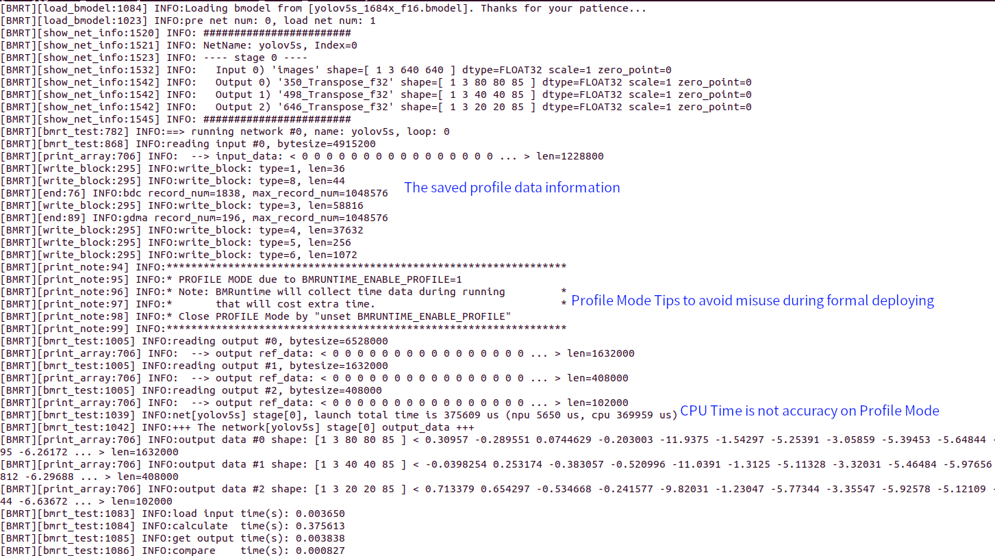
At the same time, bmprofile_data-1 folder will be generated in the current path, including all the profile data
4. Visualize Profile Data#
tpu-mlir provides tpu_profile.py script,that can convert the raw profile data to a web page file, to visualize the data.
The command is used as follows:
1 | Convert the data in bmprofile_data_0 folder to a web page in bmprofile_out |
Open bmprofile_out/result.html with web browser to show the profile chart
The more usage can be shown by tpu_profile.py --help.
5. Analyse the Result#
5.1 Overall Introduction#
The complete page can be roughly divided into instruction timing chart and memory space-timing chart. By default, the memory space-timing chart is collapsed and needs to be expanded through the checkbox “Show LOCALMEM” and “Show GLOBAL MEM”.
Below, we will explain how to analyze the running status of TPU for these two parts separately.
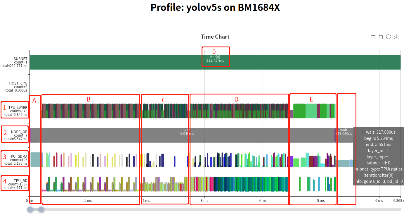
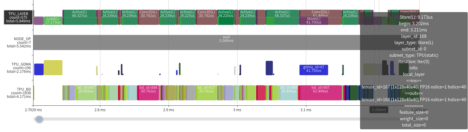
The above chart is an instruction timing chart, which is explained by the labels in the chart as follows
When creating a profile, the time on the host may not be accurate, and this section is only used as represent subnet separation markers.
This line represents the timing of each Layer in the entire network, which is derived by the following TPU_GDMA, TPU_BD (TIU) actual operations. A
Layer Groupdivides an operator into two parts: data transmission and computation, and runs in parallel. Therefore, half-height color blocks are used to represent data transmission, while full height represents computation to avoid overlap.This line represents the operations on MCU, and the key functions recorded include setting GDMA, TIU instructions, and waiting for completion. The sum time of all functions in the line represents the complete actual running time.
This line represents the timing of GDMA operations in TPU. The height of the color block represents the actual data transmission bandwidth used.
This line represents the timing of TIU operations in TPU. The height of the color block represents the effective utilization rate of the calculation.
In NODE_OP line, the statistic ‘total=5.542ms’ indicates that the entire network running time is 5.542ms. It can also be seen that instructions configuration only costs a very short time and most of the time is waiting during the network execution.
The overall operation process can be divided into three parts: section A, section B-E, and section F. Among them, segment A uses MCU to move input data from user space to computational instruction space; The F segment uses MCU to move the output data from the computational instruction space back to the user space. The following mainly explains the calculation process of the B-E segment.
Readers familiar with TPU MLIR should be aware that a complete network is not run layer-by-Layer. In the middle of the network, multiple layers will be fused based on hardware resources and scheduling relationships, separating loading, computing, and saving. Unnecessary data transmission will be removed among layers in the network, called as a Layer Group, which will be divided into multiple Slices for periodic operation. The entire network may be divided into multiple Layer Groups based on its structure. We can observe the Layer Patterns of segments B, C, and D, with half height loading and saving operations in the middle and a certain period of some pattern. Based on these, we can determine that B, C, and D are three fused Layer Groups. Moreover, there is no obvious period in the later E segment, and these layers are Global Layers that have not been fused.
Overall, only 20% of the network is not fused, and at this level, the network structure is friendly to AI compiler (TPU-MLIR).
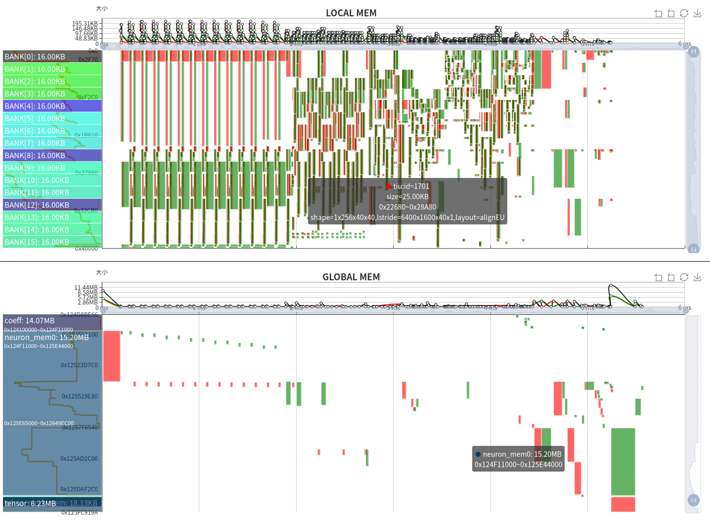
The above figure is the overall memory space-timing chart, including the upper and lower parts of LOCAL MEM and GLOBAL MEM. The horizontal axis represents time, which can be seen in conjunction with the instruction timing chart above. The vertical axis represents the range of memory space. The height of the green block in the figure represents the size of the occupied space, the width represents the length of the occupied time, in addition, red represents GDMA write or TIU output, and green represents GDMA read or TIU input.
Local MEM is the internal computing space of TPU. For BM1684X, TIU has a total of 64 lanes, each of which can use 128KB of memory and is divided into 16 banks. Since the operations of each Lane are consistent with local memory, only the local memory usage of Lane0 is shown in the figure. During the calculation process, it is also important to note that the input and output of the calculation should not be on the same bank, as data read and write conflicts can affect calculation efficiency.
GLOBAL MEM has a relatively large space, usually within the 4GB-12GB range. For ease of display, only the space blocks used during runtime are displayed. Since only GDMA can communicate with GLOBAL MEM, green represents GDMA’s read operation and red represents GDMA’s write operation.
From the memory space-time chart, it can be seen that for the Layer Group, the use of Local Mem is also periodic; The input and output of TIU are usually at each bank boundary and do not conflict with others. In terms of this network alone, Local Mem occupies relatively even space and is distributed throughout the entire range. From the spatiotemporal map of GLOBAL MEM, it can be seen that when running as a Layer Group, there are relatively fewer data write operations and more data read operations. When the Global Layer runs, it will go through “Writeback->Read->Writeback->…” during execution.
In addition, you can also see the details of the GLOBAL MEM space usage during runtime, which can be decomposed into 14.07MB for Coeff, 15.20MB for Runtime, and 6.23MB for Tensor.
5.2 Global Layer#
Below, we will analyze using a relatively simple Global Layer. Based on the Layer information, the previous layer of Cast cannot be fused with other operators due to being Permute (not shown in the figure).
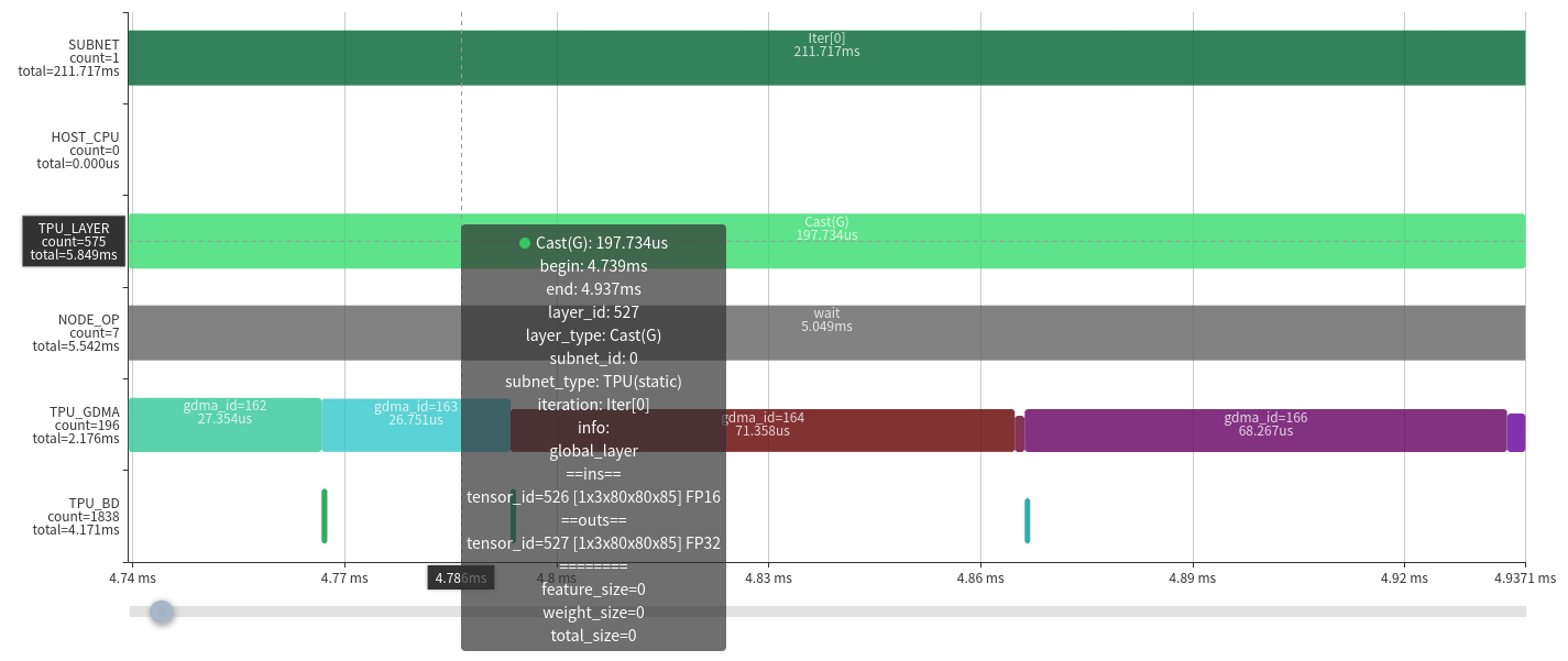
We can obtain the parameters of each layer from the chart, and the function of the current layer is casting the float16 tensor with 1x3x80x80x85 shape to float32.
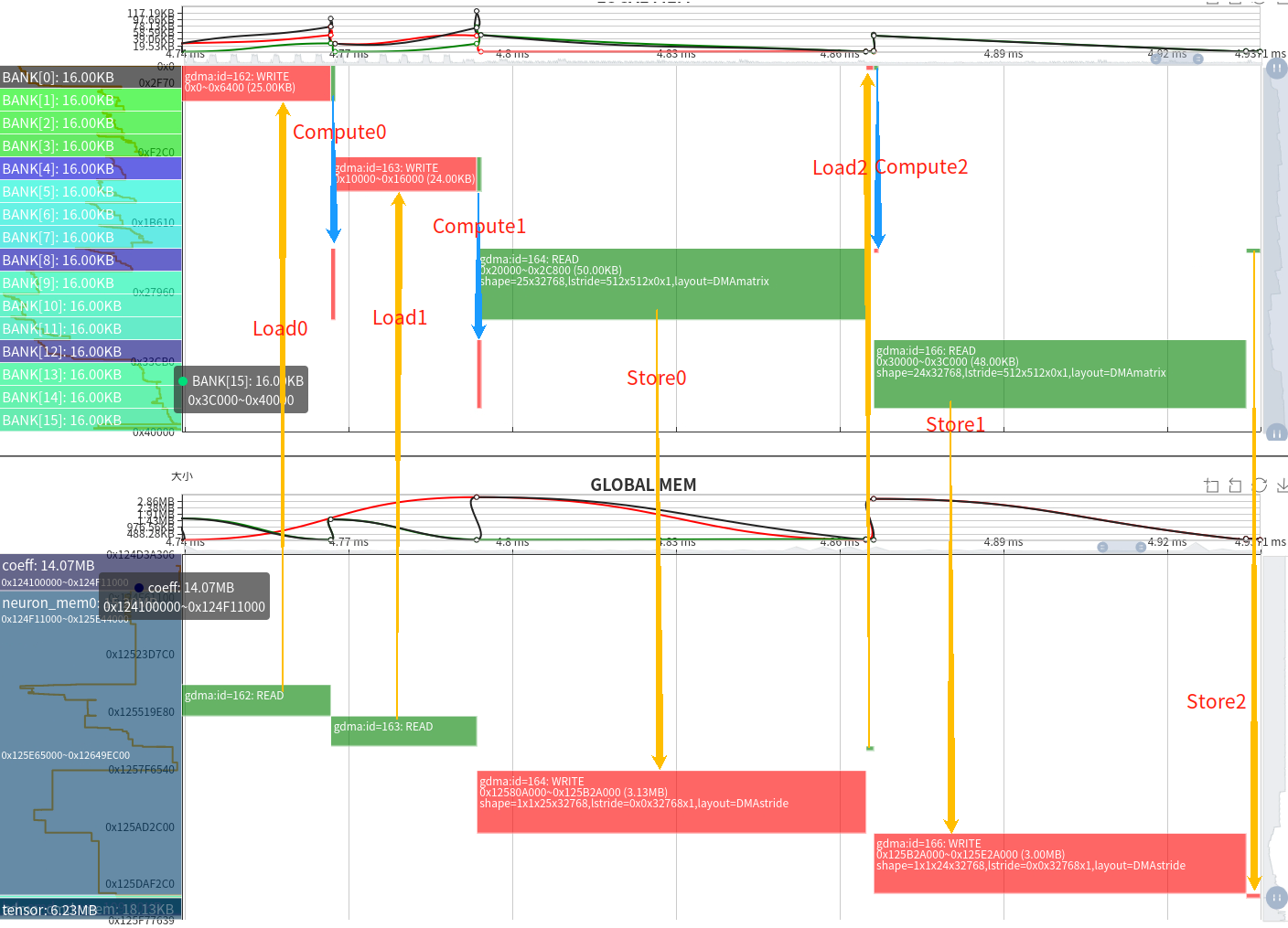
The whole process is as follows:
1 | time ---------------------------------------> |
Because there is only one GDMA device, Load operation and Store operation can only be handled serially, then the pipeline is change to:
1 | time ---------------------------------------> |
The complete data flow relationship can also be seen from the corresponding memory space-timing chart. After converting the input data from fp16 to output fp32, the memory doubled, resulting in a transmission time approximately twice that of the original.
Although pipeline parallelism has been achieved in the calculation process, due to bandwidth limitations, it cannot meet the needs of computing power. Therefore, the entire running time depends on the time when data is moved in and out. On the other hand, it also demonstrates the necessity of layer fusion.
5.3 Local Layer Group#
Based on the situation of the Layer Group above, it can be analyzed into two cases:
- High efficiency situation。The pattern is
Except for the front and back, there are only a few GDMA operations in the middle, significantly reducing the amount of data moved in and out.
TIU operation efficiency is relatively high, almost all computing power is effective
There is no gap between TIU operations (also because GDMA transmission time is relatively short)
In this case, the space for improvement is very limited and can only be optimized from network structure or other aspects.
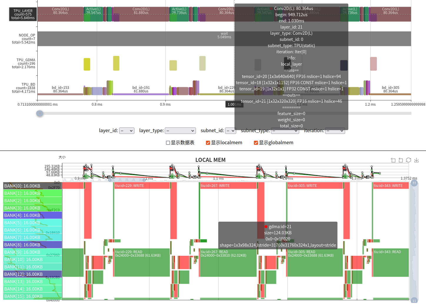
- The utilization rate of computing power is relatively low. This situation is mainly caused by the unfriendly network operator parameters with our TPU architecture. Our BM1684X has 64 lanes corresponding to the input IC, which means that the input IC is a multiple of 64 to fully utilize the Conv atomic operation of the TIU. But from the parameters in the figure, it can be seen that the input channel of the network Conv is 3, resulting in only 3/64 of the effective calculation.
When encountering unfriendly parameters, there are the following solutions:
Make full use of LOCAL MEM to increase Slice and reduce the number of instructions;
Utilize some transformations, such as data permutation, to fully utilize TPU. In fact, for the case where the input channel of the first layer is 3, we have introduced a 3IC technology to solve the problem of low computational efficiency;
Modify the original code and adjust the relevant calculations.
In practice, we have also encountered many unavoidable inefficiencies, which can only be solved by improving the TPU architecture or instructions as we gradually deepen our understanding of TPU computing.
##6 summary
This article demonstrates the complete process of profiling TPU and introduces how to use the visualization chart of the profile to analyze the running process and problems in TPU.
The Profile tool is a necessary tool for us to develop AI compilers. We not only need to analyze and think about optimization methods and methods in theory, but also need to observe the bottlenecks in the calculation process from the perspective of what happened inside the processor, providing in-depth information for software and hardware design and evolution. In addition, the Profile tool also provides a debugging way for us, allowing us to visually detect errors, such as memory overlapping, synchronization errors, and other issues.
In addition, the display function of TPU Profile is continuously improving, and any valuable feedback is welcomed.